Trading Part 2: Validation
Preview: Modeling Trends
I’ve read a whole host of papers on this topic and one of the more accessible models for market trends that I’ve come across is to adapt the concept of Geometric Brownian Motion (GBM) from molecular physics. In a nutshell we assume that day-to-day returns follow a martingale/random walk process with drift:
dS = µSdt + σSdW
Where:
- dS is the differential value of S (change of S)
- σ (sigma) is the volatility
- µ (mu) is the drift
- dt is the differential time (the time step)
- W is the so-called Wiener process, representing the aforementioned random walk
In order to capture volatility smile it’s not uncommon to use a stochastic volatility model (Heston’s is popular and not so difficult to implement from scratch) wherein we consider that the vol is itself subject to a random walk, and that the volatility of returns is related to the “volatility of the volatility” (lol) by an empirically-determined correlation factor, usually denoted as ρ (rho). The difficulty in implementing a Heston model is actually in the calibration and ongoing re-calibration of the model because there are several parameters that need to be estimated.
In any case we’re not going to get into Heston here. Instead I’m going to examine some data in order to validate some assumptions I made in Part 1.
Are mean returns zero?
I grabbed a quick CSV file of the S&P 500 daily closes for calendar year 2018. With some lisp and a little razzle-dazzle we can compute the logarithmic daily returns:
  (lisp-stat:defdf spx (lisp-stat:read-csv #P"./sp500.csv"))

  (defun logret-vector (input)
    (let ((v (make-array 1 :fill-pointer 0)))
      (vector-push-extend 0.0 v)
      (loop for i from 1 below (length input)
	    do (vector-push-extend (- (log (elt input i)) (log (elt input (- i 1)))) v))
      v))

  (lisp-stat:add-column! spx 'logret (logret-vector (lisp-stat:column spx 'close)))
Essentially what I’ve done here is instantiate an expandable vector and destructively added it to the data frame as a column. Then, we can use subseq to grab arbitrary chunks of time and determine the mean logarithmic return over the specified time frame:
(lisp-stat:mean (subseq spx 3 8))
All’s well there, so let’s take two random indices within the vector and compute the mean, and we’ll do that ten thousand times. Each iteration, we’ll collect the mean to a list of means, and then we’ll compute a “mean mean return”:
  (let ((col (lisp-stat:column spx 'logret)))
    (lisp-stat:mean (loop for i from 0 to 10000
			  for a = (random (length col))
			  for b = (random (- (length col) a))
			  collect (lisp-stat:mean (subseq col a (+ a b))))))
Evaluating this in my REPL gives a mean return of about -0.001% depending on how the RNG decides to give out integers. I’m comfortable calling anything less than a tenth of a percentage point effectively zero.
How does Realized Volatility trend?
The second assumption I want to validate is the degree to which realized volatility varies from period to period. I’m not aware of a better technique for estimating tomorrow’s realized vol than by taking a simple moving average of N periods of historical vol, but if you know of one then please get in touch with me because I’d love to hear from you.
Realized volatility is the square root of realized variance, which, since we are assuming the mean is equal to zero for simplicity’s sake, is just the sum of squared logarithmic returns:
  (let ((col (lisp-stat:column spx 'logret)))
    (sqrt (reduce #'+ (map 'vector
			   (lambda (x) (expt x 2))
			   (subseq col 51 251)))))
If you annualize the result of this calculation it comes out to about 17% and I want to make it clear at this point that the VIX is calculated in a completely different way (it’s done using call and put prices) so this number won’t be comparable to predictions made from the VIX.
In any case, the annualized figure compares quite favorably with some analysis done by Nasdaq GIS (pdf warning), so I like this result.
Given the above, we can take successive windows of, say, 200-day realized vol and see what the differences are:
  (let ((col (lisp-stat:column spx 'logret)))
    (loop for a from 51 downto 0
	  for b = (+ a 200)
	  collect (sqrt
		   (reduce #'+
			   (map 'vector
				(lambda (x) (expt x 2))
				(subseq col a b))))))
The above snippet produces a list of 200-day realized volatilities, and if we compare their percentage-differences and plot the results we can see that the vast majority of the time, volatility is within 2% of the previous day’s value!
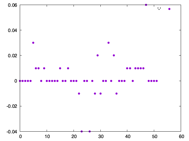
In the pathological cases for calendar year 2018 we saw changes by up to 6% close-to-close, but in general I’d say it’s safe to conclude that the trailing 200-day realized vol is a strong predictor of tomorrow’s realized vol. In part 3 we’ll put some of these concepts into practice when we forecast returns using statistics. See you next time!